<?xml version="1.0" encoding="utf-8"?><feed xmlns="http://www.w3.org/2005/Atom" ><generator uri="https://jekyllrb.com/" version="3.10.0">Jekyll</generator><link href="https://vaghawan.github.io/feed.xml" rel="self" type="application/atom+xml" /><link href="https://vaghawan.github.io/" rel="alternate" type="text/html" /><updated>2026-02-10T03:09:35-08:00</updated><id>https://vaghawan.github.io/feed.xml</id><title type="html">Vaghawan</title><subtitle>Wandering through and through..</subtitle><author><name>Vaghawan Ojha</name><email>none@example.org</email></author><entry><title type="html">Upper Bounds and So on ..</title><link href="https://vaghawan.github.io/mathematics/upper-bounds-analysis/" rel="alternate" type="text/html" title="Upper Bounds and So on .." /><published>2025-12-09T02:18:00-08:00</published><updated>2025-12-09T02:18:00-08:00</updated><id>https://vaghawan.github.io/mathematics/upper-bounds-analysis</id><content type="html" xml:base="https://vaghawan.github.io/mathematics/upper-bounds-analysis/"><![CDATA[<h2 id="upper-bounds-and-so-on-">Upper Bounds and So on ..</h2>

<p>You may be thinking that this is going to be a deep mathematical stuffs, but unfortunately no! This is going to remain as simple as possible</p>

<p>We’re acutely aware and some of us may rather be thrilled with the following expression:</p>

<p>A <strong>function</strong> $f:X\rightarrow \mathbf{R}$ is bounded above on $X$ if and only if $\exists M \in \mathbf{R}$ s.t. $f(x)\le M$. (i)</p>

<p>For a very long time, I was stuck at this very point of analysis. As most students have the same feeling about epsilon and delta, I too just wanted to manage and get away, at least for the sake of exams.</p>

<p>Then after many years I found the book, <strong><em>How to Analysis</em></strong> by Lara Alcock. I can’t emphasize how the book shaped my understanding of analysis, even only in first few pages.</p>

<p>The above definition is something that I literally copied from the book. First of all, it is also important that we know to put this definition into plain words.</p>

<hr />

<p>The equation (i) we saw above means:</p>

<blockquote>
  <p>“A <strong>function</strong> $f$ from the set $X$ to the reals is bounded above on $X$ if and only if there exists $M$ in the reals such that for all $x$ in $X$, the function $f(x)$ is less than or equal to $M$”.</p>
</blockquote>

<p>This definition basically defines a property of a <strong>function</strong> $f$, from set $X$ to reals. This is also written as $f: X \rightarrow \mathbf{R}$. $f$ takes $x$ as inputs and outputs the real numbers. One thing that we must realize at this point is that this function is defined for every real number, so the domain of this function is $X=\mathbf{R}$.</p>

<p>To see whether or not this function is bounded above, we need to check whether or not this definition is satisfied.</p>

<hr />

<p>Let’s concretize this abstract function $f$ into something simpler and familiar: $f(x)=x^{2}$.</p>

<p>Now for $f(x)=x^{2}$ to be bounded above on $f: \mathbf{R}\rightarrow \mathbf{R}$, $\exists M\in \mathbf{R}$ such that $\forall x\in \mathbf{R}$, $x^{2}\le M$.</p>

<p>
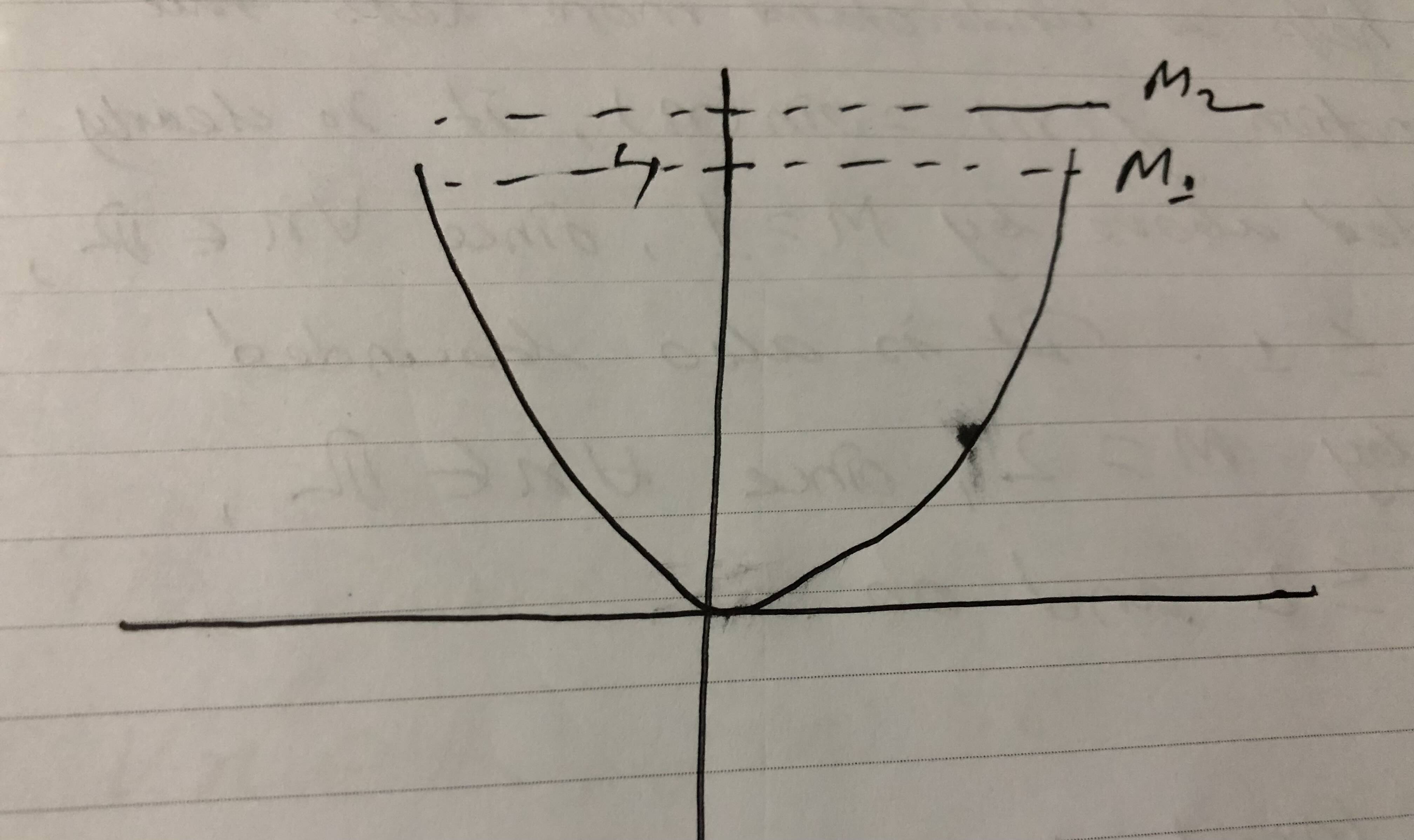
Now, let’s plot this function. Let’s take any arbitrary point $M$. Does it satisfy the condition $f(x) \le M$?</p>

<p><img src="/images/fx-image-1.jpg" alt="function of x squared" /></p>

<p>
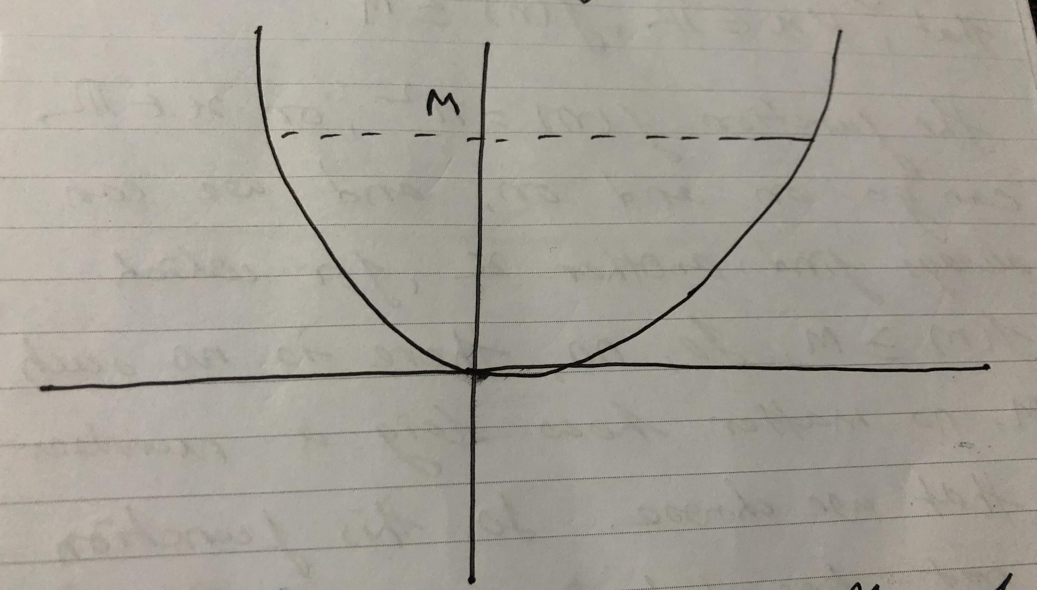
Let’s take any arbitary point $M$, does it satisfies the condition $f)x) \leq M$?</p>

<p>In other words, we need to check whether values in the vertical axis are less than or equal to $M$. 
Clearly, in our figure, the choosen $M$ does not satisfy this condition.</p>

<p>However, we’re broadly interested in knowing whether there exists such $M$ such that $f(x) \le M$ , $\forall x \in \mathbf{R}$. 
The function $f(x) = x^2$, on $X \in \mathbf{R}$, can go on and on, and we can always find another $x$, for which $f(x) &gt; M$. So, no, there is no such $M$, no matter how large a $M$ that we choose.</p>

<p>So, this function is <strong>not bounded above</strong> particularly on this domain $X=\mathbf{R}$.</p>

<hr />

<h3 id="domain-restriction">Domain Restriction</h3>

<p>But does that also mean $f(x) = x^2$ is never bounded above?
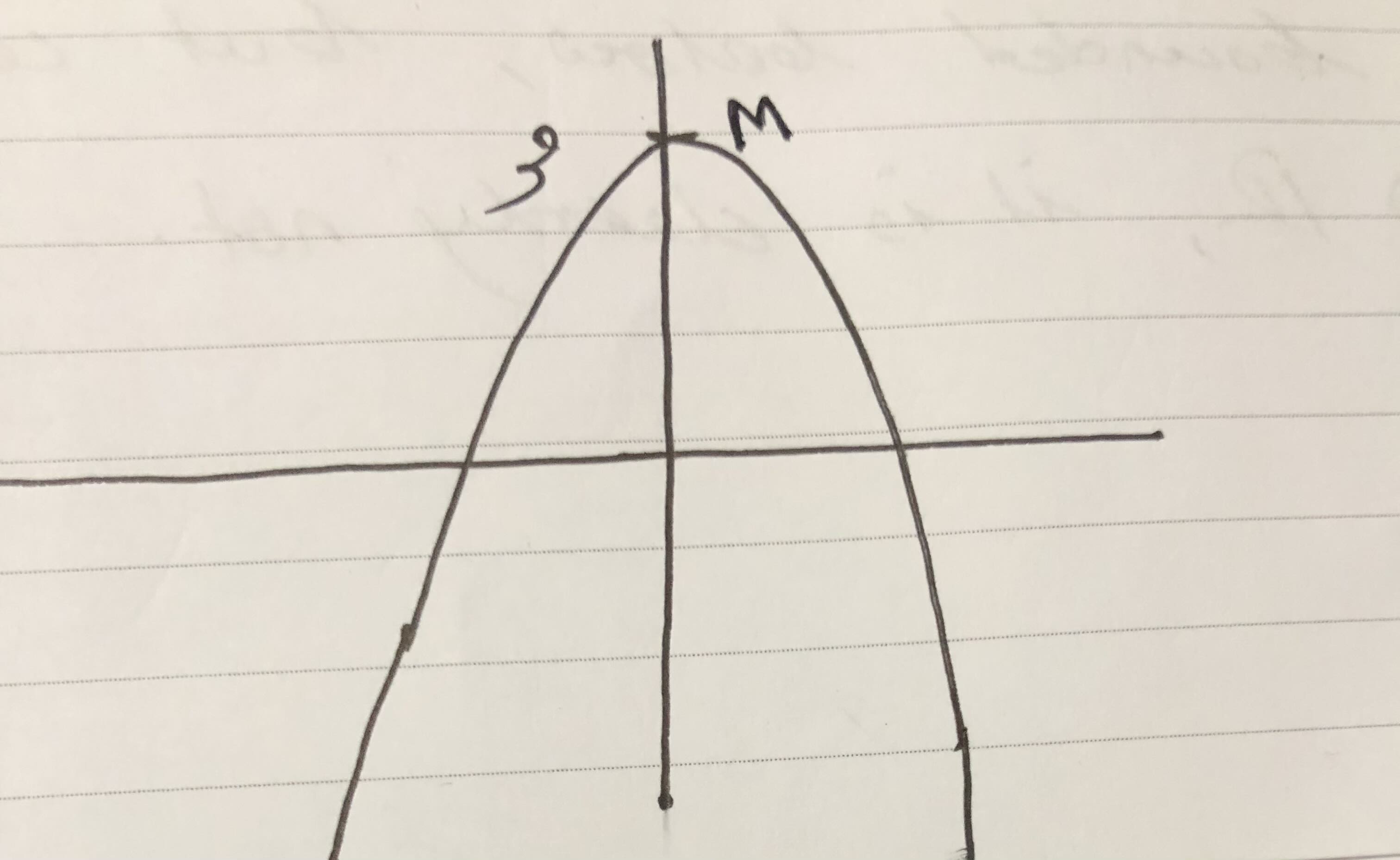
</p>

<p><strong>No!</strong> Let’s say we choose a domain $X \in [0, 2]$.
We then plot the function $f(x)=x^{2}$ again. , showing $M=4$ as an upper bound.</p>

<p><img src="/images/fx-image-2.jpg" alt="function of x squared" /></p>

<p>As we can see, in this domain, clearly when we choose $M \ge 4$, the function $f(x)$ is <strong>bounded above</strong>.</p>

<p>Another thing to notice here is that any values greater than or equal to 4 will work. That means there can be as many $M$ and it doesn’t necessarily have to be a single value as our definition does not complain about that explicitly or neither say a perfect bound.</p>

<hr />

<h3 id="example-2-fx--sinx">
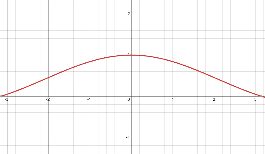
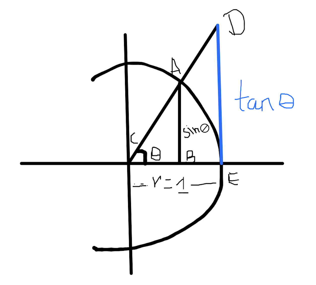
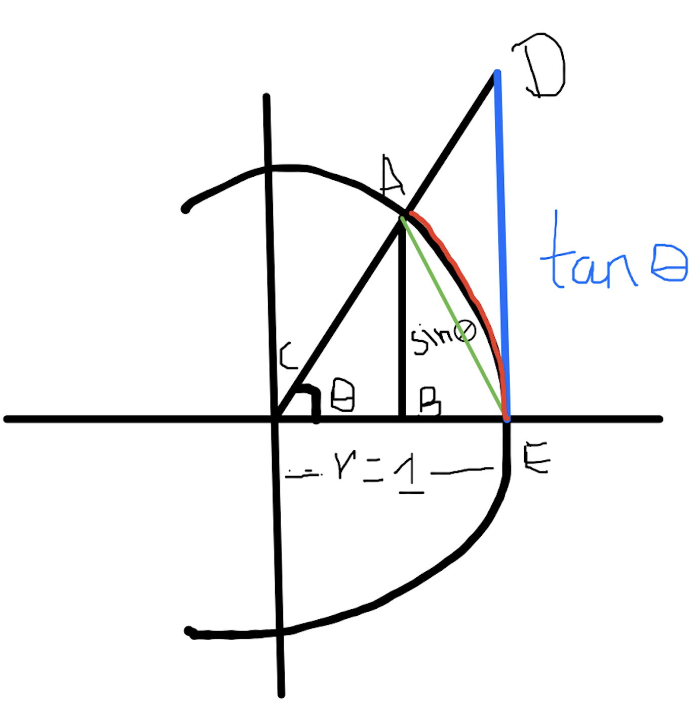
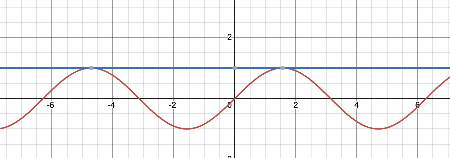
Example 2: $f(x) = \sin(x)$</h3>

<p>To help us understand more, let’s take a function $f(x) = \sin(x)$. It is clearly <strong>bounded above</strong> by $M \ge 1$. It is also bounded above by $M=2$, since $\sin(x) \le 2$ and so on.</p>

<p><img src="/images/fx-sinx-image-3.png" alt="function of sin(x)" /></p>

<hr />

<p>Now, let’s consider the function $f(x) = 3-x^2$. As you can imagine, this is clearly <strong>bounded above by 3</strong>.</p>

<p>But what about <strong>bounded below</strong>?</p>

<p>This is a little exercise question that the book poses: could you write down a definition of <strong>bounded below</strong> and confirm this?</p>

<p>So, let’s write that in fact:</p>
<blockquote>
  <p>A <strong>function</strong> $f: \mathbf{R} \rightarrow \mathbf{R}$ given by $f(x) = 3-x^{2}$ is <strong>bounded below</strong> in $\mathbf{R}$ if and only if $\exists m \in \mathbf{R}$ s.t. $\forall x\in \mathbf{R}$, $f(x) \ge m$.</p>
</blockquote>

<p>So, as you can notice, 3 is the upper bound of this function. We can <strong>not find any $m$</strong> such that $f(x)\ge m$. For the function $f(x) = 3-x^{2}$, it goes on and on with the negative values in the vertical axis.</p>

<p><img src="/images/fx-image-3.jpg" alt="function of 3 - x squared" /></p>

<p>So, while this function is <strong>bounded above</strong> ($f(x) \le 3$), this function is <strong>not bounded below</strong>, as there is no $m$ to satisfy the definition.</p>

<p>Again, if we <strong>restrict the domain</strong>, then we can definitely have the function <strong>bounded below</strong>, but when $X = \mathbf{R}$, it is clearly not.</p>

<h2 id="references">References</h2>

<ol>
  <li><a href="https://www.amazon.com/Think-About-Analysis-Lara-Alcock/dp/0198723539">How to Think About Analysis by Lara Aclock</a></li>
</ol>]]></content><author><name>vaghawan</name></author><category term="mathematics" /><category term="mathematics" /><category term="analysis" /><summary type="html"><![CDATA[Upper Bounds and So on ..]]></summary></entry><entry><title type="html">Mandelina Randomization and How to..</title><link href="https://vaghawan.github.io/computational-biology/mandelian-randomization/" rel="alternate" type="text/html" title="Mandelina Randomization and How to.." /><published>2024-10-30T03:18:00-07:00</published><updated>2024-10-30T03:18:00-07:00</updated><id>https://vaghawan.github.io/computational-biology/mandelian-randomization</id><content type="html" xml:base="https://vaghawan.github.io/computational-biology/mandelian-randomization/"><![CDATA[<h2 id="mandelina-randomization">Mandelina Randomization</h2>

<p>Mandelian randomization is a method to study the casual relationship between the risk factors and the disease using genetic varitions resposible for affecting the risk factors. One common and popular classic example is</p>

<blockquote>
  <p>Does higher C-reactive protein (CRP) levels increase the risk of developing coronary artery disease (CAD)?</p>
</blockquote>

<p>Here, by using CRP gene as genetic variant, we want to study weather or not the CRP gene is associated with the risk of developing CAD. If CRP gene associates with both the blood CRP levels and the cornoary heart disease, then we say that, “Yes!”, it seems CRP is associated with the CAD. Or more scientifically, “higher CRP is a risk factor for CAD”. 
This can be illustrated using the following diagram:</p>

<p><img src="/images/Mandelian-Randomization-Graph-first.png" alt="Mandelian Randomization Graph" /></p>]]></content><author><name>vaghawan</name></author><category term="computational-biology" /><category term="data-science" /><category term="data-analysis" /><category term="computational-biology" /><summary type="html"><![CDATA[Mandelina Randomization]]></summary></entry><entry><title type="html">Squeeze Theorem and the calculation of Limit of Difficult Functions</title><link href="https://vaghawan.github.io/mathematics/squeeze-theorem/" rel="alternate" type="text/html" title="Squeeze Theorem and the calculation of Limit of Difficult Functions" /><published>2024-09-12T03:18:00-07:00</published><updated>2024-09-12T03:18:00-07:00</updated><id>https://vaghawan.github.io/mathematics/squeeze-theorem</id><content type="html" xml:base="https://vaghawan.github.io/mathematics/squeeze-theorem/"><![CDATA[<h2 id="squeeze-theorem">Squeeze Theorem</h2>

<p>As the name suggests, the Squeeze Theorem is actually quite an useful theorem to find the limit of a function that is squeezed between two other functions, given they meet certain properties.</p>

<p>Let’s take an analogy of three runners in a running track. Runner 1 (\(R_1\)), starts at the lowest track, Runner 2 (\(R_2\)), starts at the middle track, and Runner 3 (\(R_3\)), starts at the highest track.</p>

<p><img src="/images/running-track-squeeze-theorem-example.png" alt="Running track analogy for squeeze theorem" /></p>

<p>Now, as they run, when they’re about to reach the peak of the running track, \(L\), both \(R_1\) and \(R_3\) are at the same position, \(L\), then by the squeeze theorem, Runner 2 (\(R_2\)) at the distance \(c\), which was running in-between \(R_1\) and \(R_3\) in some open interval \((a, b)\) such that \(c\in (a, b)\) must also be approaching the same position, \(L\) as the distance approaches \(c\).</p>

<p>Now, that was an hypothetical analogy, Now, Let’s imagine a more mathematical scenario:</p>

<p><img src="/images/squeezed-functions.png" alt="Graph of squeezed functions" /></p>

<p>The above figure shows three functions satisfying the following condition:</p>

\[f(n) \leq g(n) \leq h(n)\]

<p>The conditions that we must meet for this theorem to be true are:</p>
<ul>
  <li>The limit of both \(f(x)\) and \(h(x)\) must exist and must approach the same value.</li>
  <li>This must hold for \(x\) in some open interval around \(c\), but this is not strictly necessary at \(c\) itself.</li>
</ul>

\[f(x) \leq g(x) \leq h(x)\]

<p>This theorem works for both one-sided and two-sided limits as long as the above conditions are met.</p>

<hr />

<p>If these conditions are met, then the Squeeze Theorem claims that as \(g(x)\) approaches \(c\),</p>

\[\lim_{x \to c} f(x) = L\]

\[\lim_{x \to c} h(x) = L\]

<p>Then,</p>

\[\lim_{x \to c} g(x) = L\]

<p>So, this means that if \(g(x)\) is sandwiched between the two functions \(h(x)\) and \(f(x)\), as \(x\) gets closer to \(c\), if both \(h(x)\) and \(f(x)\) approach the same value \(L\), then \(g(x)\) must also approach \(L\).</p>

<hr />

<p>Squeeze theorem is simple but very powerful tool when it comes to variety of situations. For example, it comes really handly when it comes to finding the limit of fundamental trigonometric functions. It is also equally useful when it comes to figuring out the limit of indeterminate forms such as \(\frac{0}{0}\) and \(\frac{\infty}{\infty}\).</p>

<h2 id="calculating-the-limit-of-lim_theta-to-0-fracsinthetatheta">Calculating the Limit of \(\lim_{\theta \to 0} \frac{\sin(\theta)}{\theta}\)</h2>

<p>When we talk about the limit of trigonometric functions, we cannot avoid the function \(\lim_{\theta \to 0} \frac{\sin(\theta)}{\theta} = 1\). 
If we were to put \(0\) in place of \(\theta\), then we would immediately get undefined limit, a division by \(0\). But if we were to plot the graph of \(\frac{\sin(\theta)}{\theta}\) vs \(\theta\), we see that as \(\theta\) approaches \(0\), the value of the function approaches \(1\).</p>

<p><img src="/images/sinx-by-x-desmos.png" alt="Graph of sinx by x" /></p>

<p>Hence, we got to thik a little deeper. 
This is one of the fundamental limits in trigonometry which is useful to calculate many other limits, which are otherwise hard to evaluate.</p>

<p>We can use the Squeeze Theorem to calculate the limit of \(\lim_{\theta \to 0} \frac{\sin(\theta)}{\theta}\) by leveraging the properties of unit circle.</p>

<p><img src="/images/limit-sinx-approaches-zero1.png" alt="Unit circle diagram for squeeze theorem" /></p>

<p>Let’s take the above unit circle sketch, the black traingle, lets call it \(ABC\), a right angled triangle. We know that the radious of the circle is \(1\), and the angle \(\theta\) is given in radians. Now, the height of the traingle, \(AB\) is the length of the line where hypotenous intersects the unit circle. And by the unit circle definition, the length of the line is going to be \(\sin(\theta)\).</p>

<p>Now, let’s consider the blue perpendicular line \(DE\), which is the opposite side of the right angled traingle \(DEC\). If we were to calculate the tangent of the angle \(\theta\), we would get the length of the line \(DE\) as:</p>

\[\tan(\theta) = \frac{\text{opposite}}{\text{adjacent}} = \frac{DE}{EC}\]

<p>We know that the adjacent side of the traingle \(EC\) is the line from the center of the circle to the point where the tangent line intersects the x-axis, which is \(1\).</p>

<p>Hence, we can say that:</p>

\[\tan(\theta) = \frac{DE}{1} = DE\]

<p>In the first quadrant, the length of the line \(DE\) is positive, but in the equivalanet fourth quadrant, the length of the line \(DE\) will be negative. Hence we can take the aboslute value of the length of the line to make sure that it is always positive. So we take \(|DE|\) to be the length of the line \(DE\).</p>

<p>Now, let’s draw anothe traingle, \(ACE\).</p>

<p><img src="/images/limit-sinx-all-traingles.png" alt="Unit circle diagram for squeeze theorem" /></p>

<p>Now, let’s calculate the area of this traningle,</p>

\[\text{Area}_{\text{ACE}} = \frac{1}{2} . base . height = \frac{1}{2} . CE . AE = \frac{1}{2} \sin(\theta)\]

<p>Now, we know that, even this larger traingle doesn’t completly cover the wedge (red colored fraction \(ACE\)) of the circle made by the hypotenuse \(AC\). From the unit circle definition, we know that the whole circle is \(2(\pi)\) radian, then this wedge covers \(\frac{\theta}{2\pi}\) of the whole circle.
Now from the area of the circle, we know that the area of the whole circle is \(\pi\), hence the area of the wedge, which is actually a smaller circle with angle \(\theta\) is \(\frac{\theta}{2\pi} . \pi = \frac{\theta}{2}\).</p>

<p>Now, let’s calculate the area of the larger traingle \(DCE\).</p>

\[\text{Area}_{\text{DCE}} = \frac{1}{2} . base . height = \frac{1}{2} . CE . DE = \frac{1}{2} \tan(\theta)\]

<p>Now, the area of the samller traingle \(ACE\) is always less than the area of the wedge also colored red \(ACE\), which is always less than the area of the larger traingle \(DCE\). Hence, we can say that:</p>

\[f(\theta) \leq g(\theta) \leq h(\theta); \\
\text{ for } \frac{\pi}{2} \leq \theta \leq \frac{\pi}{2}\]

<p>In the above statement, \(f(\theta)\) is the area of the smaller traingle \(ACE\), \(g(\theta)\) is the area of the wedge \(ACE\), and \(h(\theta)\) is the area of the larger traingle \(DCE\).</p>

<p>Substituting the values of the areas, we get:</p>

\[\frac{1}{2} \sin(\theta) \leq \frac{1}{2} \theta \leq \frac{1}{2} \tan(\theta)\]

<p>Dividing the whole inequality by \(\frac{1}{2}\), we get:</p>

\[\sin(\theta) \leq \theta \leq \tan(\theta)\]

\[\sin(\theta) \leq \theta \leq \frac{\sin(\theta)}{\cos(\theta)}\]

<p>Now, let’s divide the whole inequality by \(\sin(\theta)\), which is always positive for \(\theta \in (-\frac{\pi}{2}, \frac{\pi}{2})\).</p>

\[1 \leq \frac{\theta}{\sin(\theta)} \leq \frac{1}{\cos(\theta)}\]

<p>Taking the reciprocal of the inequality, we get:</p>

\[1 \geq \frac{\sin(\theta)}{\theta} \geq \cos(\theta)\]

<p>Now, as \(\theta\) approaches \(0\), \(\cos(\theta)\) approaches \(1\). Hence, by the Squeeze Theorem, we can say that:</p>

\[\lim_{\theta \to 0} 1 \geq \lim_{\theta \to 0} \frac{\sin(\theta)}{\theta} \geq \lim_{\theta \to 0} \cos(\theta)\]

\[1 \geq \lim_{\theta \to 0} \frac{\sin(\theta)}{\theta} \geq 1\]

\[\lim_{\theta \to 0} \frac{\sin(\theta)}{\theta} = 1\]

<p>This is the beauty of the Squeeze Theorem, which made it possibly to intituvely evaluate the limits of \(\lim_{\theta \to 0} \frac{\sin(\theta)}{\theta} = 1\).</p>

<hr />

<p>To Do : Proof of the Squeeze Theorem</p>

<h2 id="references">References</h2>

<ol>
  <li>
    <p>Khan Academy. (n.d.). <a href="https://www.khanacademy.org/math/differential-calculus/dc-limits/dc-squeeze-theorem/v/squeeze-sandwich-theorem">Squeeze (sandwich) theorem</a>.</p>
  </li>
  <li>
    <p>Khan Academy. (n.d.). <a href="https://www.khanacademy.org/math/differential-calculus/dc-limits/dc-squeeze-theorem/v/sinx-over-x-as-x-approaches-0">Sinx/x as x approaches 0</a>.</p>
  </li>
</ol>]]></content><author><name>vaghawan</name></author><category term="mathematics" /><category term="mathematics" /><category term="calculus" /><summary type="html"><![CDATA[Squeeze Theorem]]></summary></entry></feed>